
How Many Power Iteration Steps do 1-Lipschitz Networks Need?
Published:
Power iteration is a widely used algorithm for constructing 1-Lipschitz neural networks. It’s a simple and efficient way to estimate the Lipschitz constant of any linear layer. However, there is an important issue: Power iteration provides a lower bound of the spectral norm at each step, and not the upper bound we actually need for robustness guarantees. This means that unless the algorithm is run to convergence, we cannot use the estimates for robustness guarantees.
In this blog post we investigate what “to convergence” really means in the context of 1-Lipschitz networks. Specifically, we ask: How many power iteration steps are required to obtain reliable guarantees?
💥 The Main Result
Let’s start with the main result first: Reliable estimates require far more steps than commonly assumed.
For example, for a standard Lipschitz architecture, to reduce the relative estimation error to \(\le 1\%\), we might actually need as many as 10,000 power iteration steps for each layer of a network. To guarantee a relative error of \(\le 10\%\), we still need at least 1,000 steps per layer.
We can also explicitly construct weight matrices where power iteration underestimates the Lipschitz constant for a long time. See the plot below for the results of running power iteration with such adversarial weight matrices.
Let’s now unpack the details behind these results.
🧮 The Math
Power iteration is designed to estimate the eigenvalue with the largest magnitude of a matrix. It starts with a random initial vector \(b_0\), and iteratively computes
\[b_k = \frac{A b_{k-1}}{\| A b_{k-1}\|_2} \quad \text{and} \quad \mu_k = b_k^\top A b_k.\]The sequence \((\mu_k)\) converges to the eigenvalue of \(A\) with the largest magnitude.
We can apply power iteration to \(A = W^\top W\) in order to find the spectral norm of a matrix \(W\), The spectral norm is equal to the Lipschitz constant of the linear map \(x \mapsto Wx\).
🐢 Why Convergence Can Be Slow
First, the power method converges to the true spectral norm only if the initial vector \(b_0\) has a non-zero component in the direction of the dominant singular vector. However, as long as we initialize \(b_0\) randomly (and not e.g. use the value obtained during training), this should not be a problem in practice.
The convergence rate on the other hand depends on the spectral gap of \(A\). It is defined as \(\lambda_1 \ / \ \lambda_2\), the ratio between the largest and second-largest singular values. If this gap is small (i.e., the top singular values are close), convergence slows dramatically. In worst-case scenarios, there is no limit on the amount of iterations required until convergence to the correct value.
Unfortunately, for trained Lipschitz networks we believe there is a high chance for worst-case scenarios to occur, since the networks are optimized “against” power iteration. As a result, we might underestimate the Lipschitz constant of our networks, leading to false guarantees of robustness.
However, not all hope is lost. For Lipschitz networks, we do not actually need the power method to converge exactly to the true Lipschitz constant. It is sufficient to ensure that the estimate is within a small margin. This tolerance still allows us to make meaningful robustness guarantees, by accounting for the potential estimation error in our bounds.
🧠 Analysing Hard Cases
In order to better understand how power iteration behaves in the worst case, we will construct a matrix in this section that power iteration struggles with.
Let the matrix dimension be \(d \times d\). We will consider the diagonal matrix \(M\), with \(M_{11} = 1\) and \(M_{ii} = 1 - \delta\) for \(2 \le i \le d\) where \(\delta\) is a small positive constant. This matrix has a largest eigenvalue of \(1\).
For simplicity, we will set the initial vector to \(b_0 = \frac{1}{\sqrt{d}}(1, \dots, 1)^\top\). Similar results should hold with high probability for random initial vectors.
With a bit of math we arrive at the following result:
In this setup, at iteration \( k \) we have $$ b_k = \frac{\left( 1,\ (1 - \delta)^k,\ \dots,\ (1 - \delta)^k) \right) ^\top}{\sqrt{1 + (d-1) (1 - \delta)^{2k}}} $$ and the estimated eigenvalue is $$ \begin{align} \mu_k &= \langle b_k,\ b_{k+1} \rangle \\ &= \frac{1 + (d-1) (1 - \delta)^{2k+1}}{1 + (d-1) (1 - \delta)^{2k}} \\ &= 1 - \delta \frac{(d-1) (1 - \delta)^{2k}}{1 + (d-1) (1 - \delta)^{2k}}. \end{align} $$ To ensure, for example, that \(\mu_k \ge 1 - \frac12 \delta\), we require $$ (d-1) (1 - \delta)^{2k} \le 1,$$ or equivalently, $$ \log(d-1) + 2k * \log(1 - \delta) \le 0,$$ Using the approximation \(1 - \delta \sim \exp(-\delta)\) for small \(\delta\), we get the requirement that $$ k \ge \frac{1}{2\delta} \log(d-1).$$ Similarly, for any \(0 < \theta < 1\), in order to get \(\mu_k \ge 1 - \theta \delta\), we require $$k \ge \frac{1}{2\delta} \log \left( (d-1) \frac{1 - \theta}{\theta} \right).$$ Writing \(\delta = \frac{\epsilon}{\theta}\), gives us the following result:For any \(\epsilon\) and any \(\theta \in [0, 1]\), if we set \(\delta = \frac{\epsilon}{\theta}\) in the matrix \(M\) defined above, we get an estimate \(\mu_k \ge 1 - \epsilon\) only when
\[k \ge \frac{\theta}{2\epsilon} \log \left( (d-1) \frac{1 - \theta}{\theta} \right).\]So we need at least that many steps of power iteration to guarantee a relative error \(\le \epsilon\).
📊 Practical Implications
In the result above we can e.g. choose \(\theta=0.9\). Then for any \(\epsilon\), to guarantee a relative error of at most \(\epsilon\), we need at least
\[\frac{9}{20 \epsilon} \log \left( \frac{d-1}{9} \right)\]steps of power iteration (and potentially even more).
For example, to estimate the Lipschitz constant of a single layer within 1%, we might require \(\ge 45 \log \left( \frac{d-1}{9} \right)\) power iterations. To get within 0.1%, this increases to \(\ge 450 \log \left( \frac{d-1}{9} \right)\).
Now consider a network with \(l\) linear layers. Since the overall Lipschitz constant can grow like the product of the layer-wise constants, we must ensure each layer’s estimate is extremely tight.
To achieve a network-level relative error of \(\epsilon\), each layer must be estimated with error approximately \(\frac{\epsilon}{l}\). More precisely, to obtain a network level relative error of \(\epsilon\), assuming equal layer errors, each layer must have a relative error smaller than \(\frac1l \log \left( \frac1{1-\epsilon} \right)\). This means the number of power iteration steps required becomes
\[\frac{9 l}{20} \log\left(\frac{1}{1-\epsilon}\right)^{-1} \log \left( \frac{d-1}{9} \right).\]Plugging in numbers from our comparison paper: If we assume \(l = 27\), \(d \sim 2^{16}\) for early convolutional layers, then guaranteeing a good estimation of the Lipschitz constant (within 1%) requires at least 10,000 steps of the power iteration per layer. Even to just guarantee a relative error of \(10\%\) needs at least 1,000 steps per layer.
This is much more steps than many current works aiming to guarantee a small Lipschitz constant do. Therefore, there is a possibility that some of these works overestimated the robustness of their networks.
🔬 Experiment: Measuring Convergence in Practice
To validate our theoretical findings, we simulated running power iteration on every layer of a network to estimate its overall Lipschitz constant. As in the theoretical analysis, we assumed \(l=27\) layers and input dimension \(d=2^{16}\). We used the same diagonal matrices \(M\). Unlike above, in our experiments, we sampled the initial vector randomly, as typical practice in power iteration.
📈 Results:
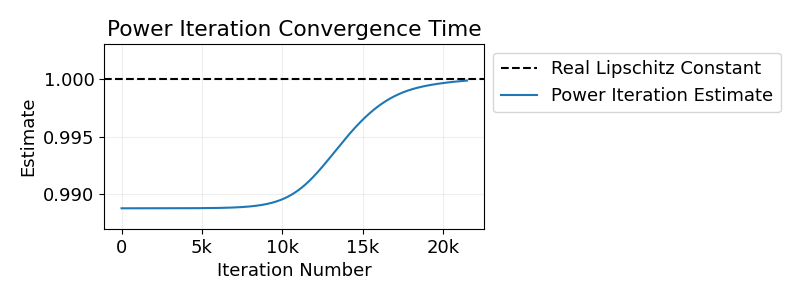
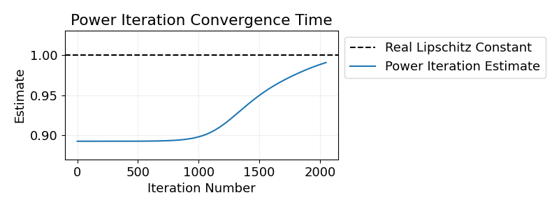
Below we show the results for two different values of \(\delta\). The findings confirm our theoretical results.
The first experiment we choose a \(\delta\) to make it difficult for power iteration to reduce the relative error below \(10\%\). And indeed, in order to get an estimate within \(10\%\) of the true Lipschitz constant, in our experiments 1,000 steps are needed.
In the second experiment, we set \(\delta\) with relative error of \(1\%\) in mind. In this case we require more than 10,000 steps of power iteration to get a relative error \(\le1\%\).
For details see our code.
😨 Could It be Even Worse?
Fortunately, not much. In particular, if we assume that the initial vector \(b_0\) for power iteration has magnitude \(t\) in the direction of an eigenvector with maximal magnitude (and \(\|b_0\|_2 = 1\)), we can show that (if \(t^2 \le 0.5\)) we need at most
\[\frac{1}{2\epsilon} \left( 1 + \log\left( \frac{1}{t^2} -1 \right) \right)\]steps of power iteration to reach a relative error of \(\epsilon\). In particular, we can convert any lower bound on \(t\) that holds with high probability, into one that bounds the relative estimation error \(\epsilon\) (after a fixed number of steps) with high probability: For any \(T^2 \le 0.5\), if \(t \ge T\) with probability \(p\), after \(k\) steps of power iteration the relative error will be
\[\le \frac{1}{2k} \left( 1 + \log\left( \frac{1}{T^2} - 1 \right) \right)\]with probability of at least \(p\).
Proof:
For this proof, WLOG we will assume that the largest eigenvalue is equal to \(1\). Suppose we are doing power iteration on a matrix \(M\) with initial vector \(b_0\), \(\|b_0\|_2=1\). We will consider a basis of eigenvector \(e_1, \dots e_d\) of \(M\) (with corresponding eigenvalues \(\lambda_1, \dots, \lambda_d\)) and define \(t_1, \dots t_d\) such that $$ b_0 = \sum_{i=1}^{d} t_i e_i. $$ Then it follows that $$ b_k = \sum_{i=1}^{d} t_i \lambda_i^k e_i.$$ Then \(\mu_k \ge 1 - \epsilon\) only if $$ \sum_{i=1}^{d} t_i^2 \lambda_i^{2k+1} \ge (1 - \epsilon) \sum_{i=1}^{d} t_i^2 \lambda_i^{2k} $$ or equivalently $$ \sum_{i=1}^{d} t_i^2 \lambda_i^{2k} (\lambda_i + \epsilon - 1) \ge 0. $$ As a lemma we will use the AM - GM inequality with \(n=2k+1\) and \(x_1 = \dots = x_{2k} = \frac{\lambda}{2k} \) and \( x_{2k+1} = (1 - \epsilon - \lambda) \) which tells us that $$ \lambda^{2k} (1 - \epsilon - \lambda) \le (2k)^{2k} \left( \frac{1-\epsilon}{2k+1} \right)^{2k+1}.$$ Remember also that we assumed WLOG that \(\lambda_1 = 1\). Using this, as well as the fact that \(\|t\|_2=1\) we have that: $$ \begin{align} \sum_{i=1}^{d} & t_i^2 \lambda_i^{2k} (\lambda_i + \epsilon - 1) \\ &= t_1^2 \epsilon - \sum_{i=2}^{d} t_i^2 \lambda_i^{2k} (1 - \lambda_i - \epsilon) \\ &\ge t_1^2 \epsilon - \sum_{i=2}^{d} t_i^2 (2k)^{2k} \left( \frac{1-\epsilon}{2k+1} \right)^{2k+1} \\ &\ge t_1^2 \epsilon - \left(1 - t_1^2\right) \left(1 - \frac{1}{2k+1}\right)^{2k+1} \frac{1}{2k} \exp( - \epsilon (2k+1)) \\ &\ge t_1^2 \epsilon - \left(1 - t_1^2\right) e \frac{1}{2k} \exp( - 2k \epsilon) \\ &\ge t_1^2 \epsilon \left(1 - \frac{1 - t_1^2}{t_1^2} e \frac{1}{2k \epsilon} \exp( - 2k \epsilon) \right) \\ \end{align} $$ This quantity is \(\ge0\) if $$ k \ge \frac{1}{2\epsilon} W \left(\frac{1 - t_1^2}{t_1^2} e \right),$$ for \(W\) the Lambert W function. In particular, since \(W(z) \le \log(z)\), this proves that it's enough to have $$\frac{1}{2\epsilon} \left( 1 + \log\left( \frac{1}{t^2} -1 \right) \right) $$ steps of power iteration to reach a relative error of \(\epsilon\). QED.We can use the result above to bound the relative error of a network with \(l\) layers. Assume each layer has relative error \(\le \frac{\epsilon}{l}\). Then power iteration estimates the Lipschitz constant with relative error at most \(\left(1 - \frac{\epsilon}{l}\right)^l \le 1 - \epsilon\).
📌 Final Thoughts
Power iteration is a simple and efficient method for estimating the Lipschitz constant of linear layers. However, the number of steps is often chosen arbitrarily. This can lead to underestimating the Lipschitz constant of networks, breaking the guarantees of robustness we aim to get with Lipschitz networks.
In this post, we showed that we do require a lot of steps of power iteration to guarantee a good estimation of the Lipschitz constant. In particular, if we want to get relative error of at most 1%, for a standard architecture we might require as many as 10,000 power iteration steps per layer.
This has serious implications for certified defenses and robustness claims in the literature. We hope that future work will take these convergence requirements into account when designing and certifying 1-Lipschitz networks.
![]()
Work done at ISTA under the supervision of Christoph Lampert.
 In our recent CVPR paper,