Hard Mining for Robust Classification

In this blog post we want to explore whether training mostly on the hardest examples allows us to fit robust networks on CIFAR-10 quicker.

Introduction

In machine learning we “teach” our models to perform tasks such as image classification by showing them many examples of the task. In supervised learning these examples usually consist of an input (e.g. an image) and the corresponding label. We usually show every example to the model many times, and we do this in a way where we present every image equally often. This seams to be a reasonable approach when training for a few epochs only, however, it seems wasteful when training models for a long time: We will present examples that the model already classifies well to the model again and again. This seems inefficient, and to make things worse with standard loss functions the gradient coming from those examples will be close to \(0\), so the model will not actually update its parameters anymore based on those examples, and we just waste time and compute on those examples.

It seems to be a more efficient approach to only show images to the model that are not yet classified correctly. This is essentially what “Hard Mining” does. Hard Mining was used e.g. for face recognition with triplet loss¹, for selecting pairs of pictures of different people that the model cannot distinguish yet. However, it is not very common for supervised training of image classifiers.

For a recent paper we aimed to robustly overfit the CIFAR-10 training set with 1-Lipschitz models. (For an introduction to 1-Lipschitz models, see e.g. ².) Unfortunately, 1-Lipschitz models tend to require a lot of update steps and a lot of training epochs to perform well. So whilst it is possible to overfit the training set by looking at every image equally often, this seems to by a suboptimal usage of resources. Therefore in this blog post we aim to explore if we can reduce the amount of training updates (and therefore training time), by being smarter about how often we use every image for training our models.

What we did

We want to create a way of using hard examples more often during training than easy ones. Luckily, we already have some intuition of which examples are hard and which are easy during training time: For every example we do know the value of the loss function for this example whenever this example is used during training. We decided to always use the examples with the highest loss function in order to form the next minibatch. We can achieve this efficiently by using a priority queue in order to keep track of the examples with the highest loss. This should barely have any computation overhead during training time, yet it allow us to mainly focus on the hard examples.

With the approach described above we do not consider the fact that the loss for all examples does change whenever we update the parameters of our model. We could regularly re-evaluate the loss for all training examples, however, this wastes some compute on additional forward passes of our model. Instead, we increase the priority of examples we have not seen in a while relative to newly added ones. This way we regularly process all our training examples, whist considering harder examples more frequently than easy ones. In practice, we achieve this by setting the priority of an examples to \(\mathop{\text{loss}}(x, y) - \alpha t\), for \(t\) the epoch number and \(\alpha = \frac{1}{10}\), and then always considering the examples with highest priority for the next training batch. With this choice, higher loss means higher priority, but the priority is also higher for example we have not seen in a while (and they were queued up a smaller value of \(t\)).

What we found

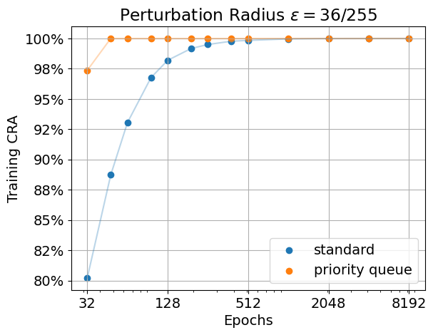
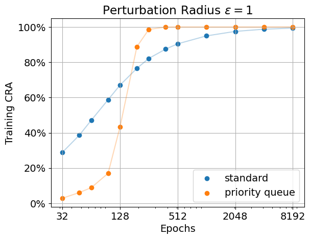
We achieve what we intended to do: Using a priority queue, we manage to fully overfit the training data robustly much quicker than with standard training. For example, for radius \(\epsilon=1\) we overfit the training data robustly in about \(256\) epochs. (Here one epoch is measured as the same number of forward passes as one epoch on standard CIFAR-10.) When showing every example equally often we require many times more compute. For the same setting as before it takes about \(4k\) epochs! See the plot below for our results. We show the certified robust accuracy (CRA) for radius \(\epsilon=36/255\) (left) and \(\epsilon=1\) (right) for a 1-Lipschitz MLP using AOL layers. We can clearly see that when focusing on the examples with the highest loss, the model first fits the data perfectly for a small radius, and then eventually increases the radius. In contrast, standard training does already fit some training examples with a large margin (\(\epsilon=1\)) after only \(32\) epochs. At the same time, there are still about \(20\)% of training examples that are not classified correctly under much smaller perturbation (radius \(\epsilon=36/255\)).

For details of our setup see e.g. our code, provided in this repository.

How about test performance?

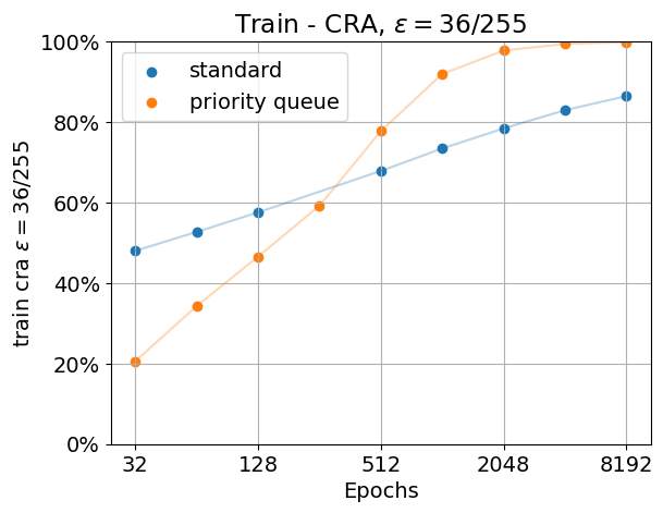
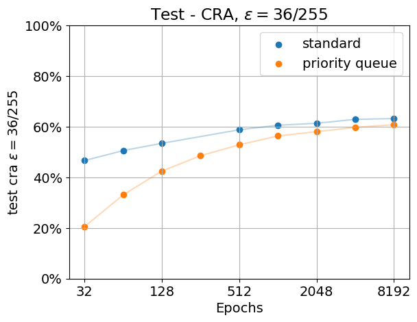
However, unfortunately the results on the training set do not transfer to the test set. There, using a priority queue does not improve performance, it actually seems to decrease the performance instead. We show the results below. We trained the model again, this time with data augmentation. When using data augmentation, overfitting the training data is harder than without, as the model never “sees” the original training images without augmentation. However, when using a priority queue, the model is still able to robustly fit all of the training data eventually. However, this comes with a price, and using a priority queue does reduce the performance on the test set in this task. This was somewhat expected: When aiming for good test set performance, overfitting the training data is usually not the best strategy.

Discussion

We have shown that when aiming to accurately fit some data, it can be useful to focus more on harder examples. We did this by using a priority queue, and training on the examples with the highest loss. As we compute the loss anyway in every model update, our method does not require additional compute. Using a priority queue allows us to overfit our training data many times quicker, however, unfortunately it does seem to decrease the test performance.