In our recent CVPR paper, “1-Lipschitz Layers Compared: Memory, Speed and Certifiable Robustness” we compared different methods of creating 1-Lipschitz convolutions. In this blog post we try to give some additional background on why 1-Lipschitz methods are an interesting research topic, and discuss some results from the paper.

Why 1-Lipschitz networks?

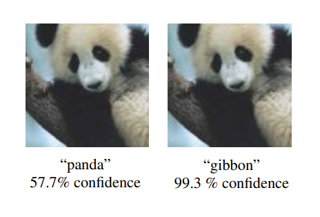
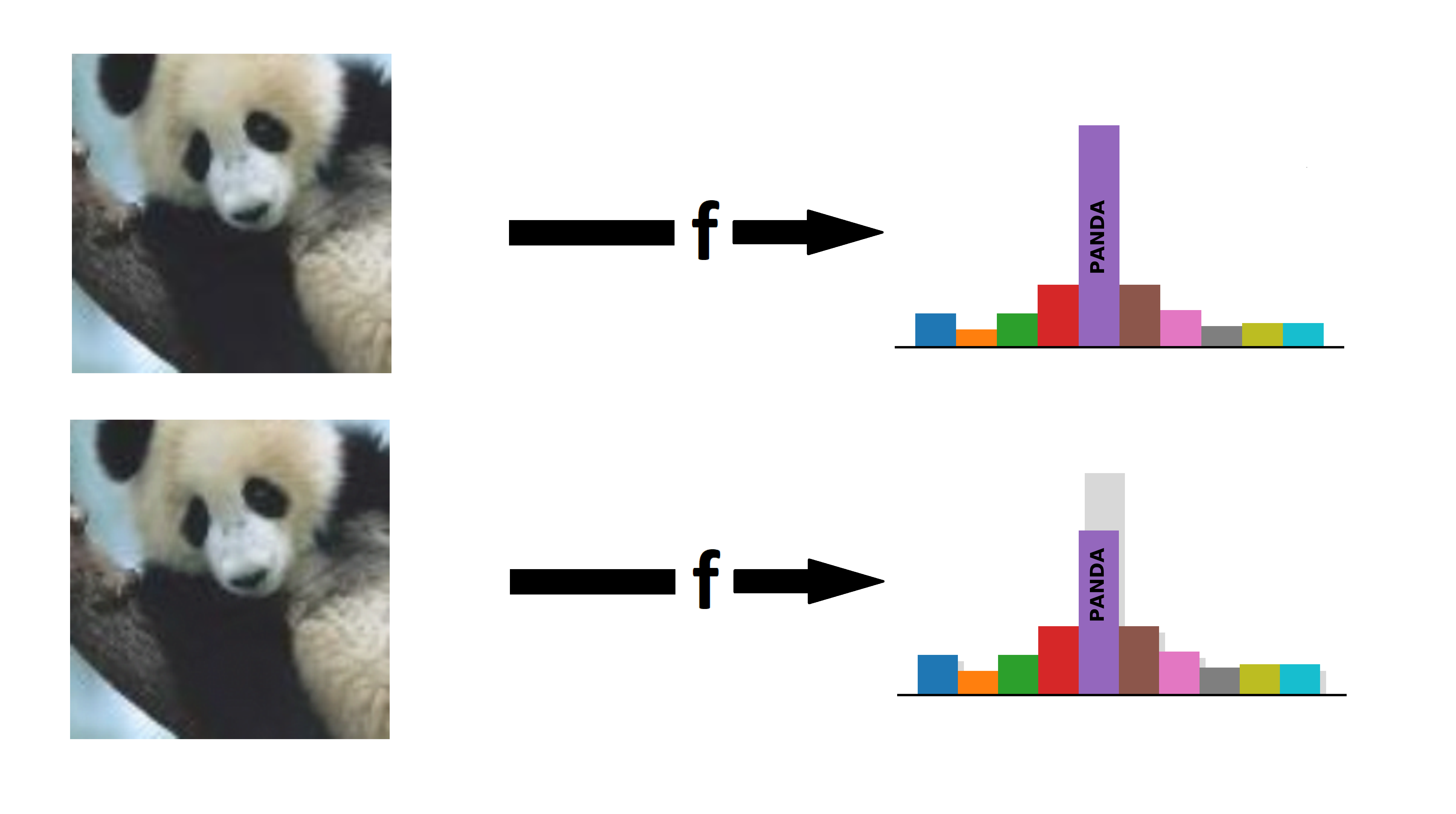
Current image classification models are not robust! Tiny, invisible perturbations of the input, known as adversarial examples¹, can change the predictions of the models.

We study adversarial example mostly to learn more about neural networks, and potentlially build models that e.g. generalize better in the future.

However, the existence of adversarial examples could also lead to some problems, such as

• users not trusting the models,
• security issues, and
• it makes it impossible to build (faithful) interpretable models.

In order to create classifiers that are guaranteed to be free of adversarial examples, many recent works have proposed methods of parameterizing 1-Lipschitz networks.

We call a function, a layer or a network 1-Lipschitz if the difference of two outputs is at most as big as the difference of the corresponding two inputs, or mathematically:

for all inputs x and y.

Once we know how to build 1-Lipschitz layers, we can simply construct 1-Lipschitz networks by stacking multiple of those layers.

When classifying an image using a 1-Lipschitz network, by construction, any perturbation of the input image can change the output of the network by at most the same amount. Therefore, if the difference of the larges 2 class scores of the original image is large enough, we can be sure that no perturbation of certain magnitude can change the order of outputs, and therefore the prediction of the model.

Existing 1-Lipschitz Convolutions

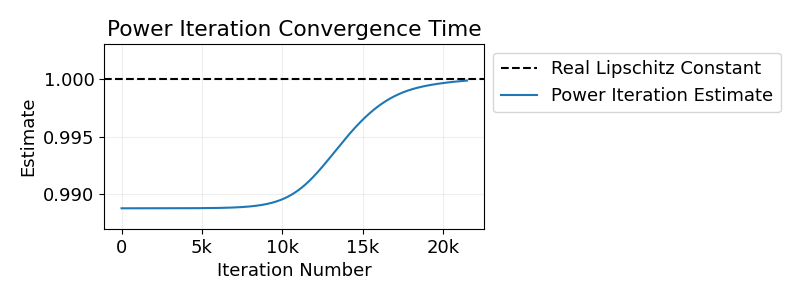
Recently, many works have tried to construct 1-Lipschitz layers. It is relatively easy to construct 1-Lipschitz fully connected layers. For example we can orthogonalize the weight matrices using a differentiable algorithm such as Björck and Bowie², or we can divide the outputs of the layer by its operator norm, obtained using power iterations. However, it is a bit more tricky to create 1-Lipschitz convolutions. For example, whilst we could apply conditions on the Jacobian of the layer, it is generally inpractical because of the size of this matrix.

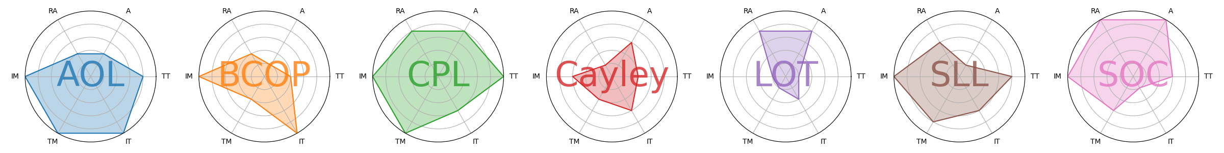
We will introduce 7 methods of creating 1-Lipschitz convolutions from the literature:

BCOP

(Li et al., 2019, NeurIPS)

The methods BCOP (Block Orthogonal Convolution Parameterization) constructs the kernel of a \( k \times k \) convolution from a set of \( (2k − 1) \) parameter matrices. Each of these matrices is orthogonalized using an algorithm by Björck & Bowie². Then, a \( k \times k \) kernel is constructed from those matrices in a way that guarantees that the resulting layer is orthogonal.

Cayley

(Trockman and Kolter, 2021, ICLR)

Cayley Convolutions make use of the fact that circular padded convolutions are vector-matrix products in the Fourier domain. As long as all those vector-matrix products have orthogonal matrices, the full convolution will have an orthogonal Jacobian. The orthogonal matrices used in this are parameterized using the Cayely Transform³: For any skew-symmetric matrix \(A\) the matrix \(Q\) is orthogonal, where \(Q\) is defined as

SOC

(Singla and Feizi, 2021, ICML)

Skew orthogonal convolutions (SOC) use an exponential convolution⁴ in order to obtain a 1-Lipschitz layer: Given a kernel \(K\), the exponential convolution can be defined as

where \(\ast^t\) denotes a convolution applied \(t\) times. The authors proved that any exponential convolution has an orthogonal Jacobian matrix as long as L is skew-symmetric, providing a way of parameterizing 1-Lipschitz layers. In their work, the sum of the infinite series is approximated by computing only the first 5 terms during training and the first 12 terms during the inference, and L is normalized to have unitary spectral norm.

AOL

(Prach and Lampert, 2022, ECCV)

We introduced Almost Orthogonal Lipschitz (AOL) as a rescaling method that guarantees a layer to be 1-Lipschitz. For a fully connected layer with a parameter matrix \(P\), we define a diagonal rescaling matrix \(D\) with

With this choice of \(D\), we show that the spectral norm of \( PD \) is bounded by 1, which implies that the the linear given by \( l(x)=PDx + b \) is 1-Lipschitz.

We can also apply this rescaling to a convolution. In order to do this we need to consider the Jacobian \(J\) of the convolution (instead of \(P\)) in the equation above. We show how to efficiently evaluate the rescaling (or more precisely an upper bound of it) by expressing the entries of \( J^\top J \) explicitely in terms of the kernel values.

LOT

(Xu et al., 2022, NeurIPS)

Layer-wise orthogonal training (LOT), relies on the fact that for any parameter matrix \(V\), the matrix \(Q = V (V^\top V)^{-1/2}\) is orthogonal. In order to evaluate this term, an iterative Newton Method is used to evaluate the inverse square root. Like Cayley convolutions, LOT parameterize 1-Lipschitz convolutions by evaluating them in the Fourier domain.

CPL

(Meunier et al., 2022, ICML)

For a parameter matrix \(P\) and a non-decreasing 1-Lipschitz function \(\sigma\) (usually ReLU), the Convex Potential Layer (CPL) is defined as

The spectral norm required to calculate \(l(x)\) is approximated using the (convolutional) power method.

SLL

(Araujo et al., 2023, ICLR)

The SDP-based Lipschitz Layer (SLL) combines the CPL with the bound on the spectral norm from AOL. The layer can be written as

where \(Q\) is a diagonal parameter metrix with positive entries and \(D\) is the AOL rescaling applied to \(P=W^\top Q^{-1}\).

Comparing 1-Lipschitz Convolutions

Theoretical

In our paper we did a theoretical comparison of different methods, considering the computational complexity and memory requirements of different methods. Our main findings where

• Doing a forward pass with any of the methods is at most a costant factor more expensive than doing a forward pass with a standard convolution.
• However, apart from CPL and SOC, all methods require some preprocessing of the parameters (e.g. orthogonalization), that usually scales like \(c^3\), for \(c\) the number of channels.
• Methods Cayley and LOT require preprocessing that furthermore depend on the input size, making those methods hard to scale to larger input sizes.
• In terms of memory required, again Cayley and LOT scale much worse with input size.

Empirical

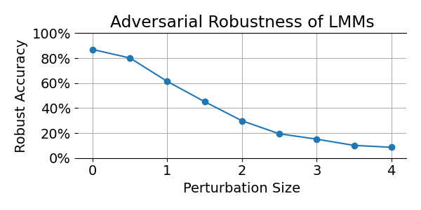
We also compared the different methods in terms of the standard tasks for 1-Lipschitz networks: Certified Robust Classification. The certified robust accuracy is the portion of the test set that is classified both correctly as well as robustly: No perturbation of certain magnitude (here \(\epsilon=36/255\)) can change the output of the model. For 1-Lipschitz networks, if for a particular input the score (=model output) for the ground truth class is at least \(\sqrt{2} \epsilon\) higher than the second largest score, then this input is classified certifyably robustly by the network. So one forward pass per image is enough to evaluate the certified robust accuracy of a model.

When training 1-Lipschitz networks, it is usually the case that the performance keeps increasing when training for longer. Also, the time required to process one epoch is very different for different models. Therefore, we decided to restrict the training time for every model, and compare them for a given time (and not epoch) budget.

In this comparison, methods CPL and SOC generally performed very well. Despite requiring a lot of resources, a LOT model reached the highest certified robust accuracy on Tiny Imagenet.

For all results and various visualizations of them check out our paper.

Interpretation

Based on our results, we believe CPL is the most promising method for creating certifiably robust models in the future.

One commonality between well performing methods that we have found is that they all either include some sort of skip connection (CPL, SLL and SOC) or initialize layers as the identity map (like AOL and LOT). We also found that as expected, doing computations on the kernel instead of on the full input is an advantage when scaling up methods to larger input resolutions. Interestingly, we did not find a large difference between layers that strictly enforce orthogonality and more general ones. Furthermore, slower methods did not seem to perform worse than faster ones; with SOC and LOT two relative slow methods are among the best ones

Please find more information and further details in our paper “1-Lipschitz Layers Compared: Memory, Speed and Certifiable Robustness”